Vibe Engines
YouTube
AI System Design

Design an LLM Inference Server

Learn AI system design by building an LLM inference serving system step by step.

The numbers to beat1 passprefill the prompt1 tokenper decode stepTTFTset by prefill

The whole design, in writing

Learn AI system design by building an LLM inference serving system step by step. An interactive guide covering the request queue, the prefill/decode split, continuous batching, the KV cache and paged attention, tensor sharding across GPUs, autoscaling on GPU pressure, and the latency-versus-throughput trade-offs of serving a model at scale.

Every step of the build above, written out: the problem each piece solves, the option that was taken and the ones that were not, the numbers, and how it fails in production.

The big idea

Why is serving an LLM hard?

Running a model once on your laptop is easy. Serving it to thousands of users at once, fast and affordably, on hardware that costs dollars per hour, is not. A single request can hog a GPU for seconds while it generates tokens one at a time. How do you keep scarce GPUs full and users’ answers fast?

Clientprompt + stream
New in this step: Client.

Treat the GPU fleet as a precious, fixed resource and design everything around it: a queue to absorb spikes, continuous batching to keep GPUs full, a KV cache to make each token cheap, sharding to fit big models, and autoscaling to ride demand.

What the new pieces do

Clientclient
Sends a prompt and reads tokens back as they stream. Cares about time-to-first-token and tokens/sec.

Step 1 · The skeleton

A client, a router, a model

A client sends a prompt and wants tokens streamed back. The model lives on GPUs that can’t be exposed directly. What sits in between?

Clientprompt + streamRouteradmit + route
New in this step: Router.

Requests arrive for a model running on a GPU fleet. What fronts it?

  1. No auth, no load balancing, no limits — and a client pinned to one worker that might be busy. You need a router in front.

  2. The router authenticates, applies limits, and sends each request to a GPU replica that has room — then streams tokens back.

  3. Generations are dynamic and rarely identical, so caching whole answers barely helps. The expensive part is fresh inference, not delivery.

A Router fronts the fleet: it admits requests, applies rate limits, and routes each to a GPU Worker with capacity, then streams the generated tokens back to the Client. The classic client → router → workers spine, tuned for streaming.

Why this piece earns its place

A router in front of a stateless service is a solved problem; in front of a stream it is not. The response stays open for as long as the answer takes, which makes the router stateful for the life of the request and breaks three defaults at once. Any buffering proxy between you and the user holds tokens until the response completes, so the server records a fast first token while the user watches a blank screen — a latency failure invisible in your own telemetry, because your own telemetry is the thing lying. Idle timeouts have to tell a long generation apart from a dead connection, which means a heartbeat, not a bigger number. And once the first token is on the wire the status code has already been sent, so a failure halfway through has to be delivered in-band, and a retry is no longer safe: the user has read part of an answer you are about to contradict. The piece to build early is cancellation. When a client disconnects, that has to reach the scheduler, or the GPU keeps decoding tokens nobody will read and reports the waste as utilization.

What the new pieces do

Routerbackend
The front door. Authenticates, applies limits, and routes each request to a model replica with capacity.

Step 2 · Absorb the spikes

Put a queue in front of the GPUs

Traffic is bursty — quiet, then a flood. GPUs are a fixed number. If requests hit workers directly, a burst either overwhelms them or, when quiet, leaves them idle. How do you smooth this?

Routeradmit + routeRequest Queueadmission
New in this step: Request Queue.

GPU count is fixed; traffic is spiky. How do you avoid stampede AND starvation?

  1. Dropping on every spike is a terrible experience and wastes capacity that frees up moments later. Buffer first, drop only as a last resort.

  2. GPUs take minutes to provision and cost too much to hold per request. You can’t scale per-request at GPU granularity in real time.

  3. A queue absorbs bursts so GPUs stay fully fed without being stampeded, and admission control can shed load gracefully when the queue gets too deep.

A Request Queue sits between the router and the GPUs. Bursts fill the queue instead of crushing the workers; in quiet moments the queue drains and GPUs stay busy. Admission control can shed load ("busy, retry") when the queue grows too deep — protecting latency for everyone already in flight.

Why this piece earns its place

A queue with no bound is not a shock absorber, it is a delay line: past a certain depth, every request that enters is already condemned to expire before a GPU reaches it. So two cheap mechanisms go in with the queue itself. A hard cap, so admission control has something to fire on. And a deadline stamped at enqueue and rechecked at dequeue, so work whose client has already given up is dropped before it buys a prefill rather than after. What admission cannot do is size the job. A request carries its prompt and a max-token cap, and that cap is a ceiling rather than a forecast — the true output length is settled only when generation stops — so every decision here is made against an upper bound and has to stay conservative about it. Two consequences worth naming. A refusal is only useful if it carries a Retry-After with jitter; a bare one returns as a synchronized wave and refills the queue you just drained. And the queue belongs in one place in front of the fleet, not as a deep inbox per replica: once a request is committed to a worker it cannot be moved, so it waits behind that worker’s longest prefill while another replica sits idle.

What the new pieces do

Request Queueservice
Holds incoming requests so the GPUs are never starved or stampeded — the buffer that absorbs spiky traffic.

Step 3 · How a token is made

Prefill, then decode

To serve a model well you have to know how it actually computes. Generating an answer isn’t one operation — it’s two very different phases with very different costs. What are they?

RouterRequest QueueGPU Workers
New in this step: GPU Workers. · swipe to pan the diagram

Generating an answer splits into two phases. What are they?

  1. Weights load once at startup, not per request. The per-request work is the two-phase prefill/decode, which dominates everything.

  2. Prefill runs the full prompt through the model in parallel (compute-heavy); decode then generates output tokens one at a time (memory-bandwidth-heavy). They scale differently.

  3. That’s a different architecture’s framing. Decoder-style LLM serving is specifically prefill (prompt) then autoregressive decode (output).

The GPU Workers do two phases. Prefill processes the entire prompt in one parallel pass (compute-bound). Decode then generates output one token per step, each step depending on the last (memory-bandwidth-bound). The asymmetry — fast parallel prefill, slow sequential decode — shapes every serving decision.

Why this piece earns its place

The reason to hold the two phases apart in your head is that they compete for the same device. A prefill is one large compute burst, and while it runs, every sequence already streaming gets no token — so one long prompt arriving mid-flight lands as a visible stutter in dozens of other people’s answers. That damage hides from both metrics named above: time-to-first-token is fine, total time is fine, and the thing that moved is inter-token latency, which almost nobody graphs. Graph it and the fixes are available — split a long prefill into chunks the scheduler interleaves between decode steps, or run prefill and decode on separate pools so the burst lands where nobody is streaming. The asymmetry also explains why the next step works at all. Decode reads the entire weight matrix to produce a single token, so running many sequences together reads those weights once instead of once each — the bandwidth that dominates the step is paid for the whole batch, not per member of it. Prefill is already compute-saturated by one long prompt, so batching buys it far less. Batching is a decode optimization.

  • 1 passprefill the prompt
  • 1 tokenper decode step
  • TTFTset by prefill

What the new pieces do

GPU Workersservice
The model running on GPUs. Does a one-time prefill of the prompt, then decodes output one token per step.

Step 4 · Keep the GPUs full

Continuous batching

Decode generates one token per step per sequence — a single request barely uses the GPU. But requests start and finish at different times and have different lengths. Naive batching wastes the GPU waiting for the slowest one. How do you keep it packed?

Batch SchedulercontinuousMetrics / ControlTTFT · tok/s · util
New in this step: Batch Scheduler, Metrics / Control.

Requests have different lengths and arrive at different times. How do you batch?

  1. A single decode step uses a fraction of the GPU; everything else waits. You’re paying for hardware that mostly idles.

  2. The whole batch stalls on the longest sequence, and new arrivals wait for the next batch. Idle gaps everywhere.

  3. A scheduler packs many sequences into each GPU step, dropping finished ones and slotting in new arrivals immediately. The GPU stays saturated regardless of length mix.

A Batch Scheduler does continuous (in-flight) batching: at each decode step it runs all active sequences together, retires the ones that just finished, and slots waiting requests in immediately — no waiting for a batch to drain. The GPU stays full no matter how lengths and arrivals mix. Serving metrics (TTFT, tokens/sec, utilization) drive its decisions.

Why this piece earns its place

Continuous batching removes the batch boundary, and that boundary was quietly doing a job: it was the moment everyone waiting got a turn. Without it, nothing in the loop is obliged to ever admit a particular queued request, so a steady arrival rate plus a few long-lived residents can hold the GPU indefinitely while a handful of requests age out at the back. Median latency looks excellent throughout, which is why this is usually found by a customer rather than a dashboard. The repair is explicit — aging, a priority that climbs with wait time, a slot reserved per step for the oldest waiter — but it has to be written, because run whatever is active contains no notion of fairness. The second surprise is that batch composition changes the output. Reductions run in a different order at a different batch size, so an identical prompt with an identical seed can produce a different token depending on who happened to be decoding alongside it. Nothing is broken. But bit-exact reproducibility is not a property this server has, and any eval that assumes it will flake forever.

What the new pieces do

Batch Schedulerservice
Packs many in-flight requests into each GPU step, adding and retiring sequences token by token.
Metrics / Controlbus
Streams serving metrics — time-to-first-token, throughput, GPU memory — that drive batching and autoscaling.

Step 5 · Make each token cheap

The KV cache and paged attention

At each decode step, attention needs to look back over every previous token. Recomputing that for the whole sequence on every single token would be brutally quadratic. And the cache that avoids it can blow up GPU memory. How do you make decode both fast and memory-efficient?

GPU Workersbatched decodeKV Cachepaged attention
New in this step: KV Cache.

How do you avoid recomputing attention over the whole prompt every token?

  1. That’s the quadratic waste the KV cache exists to kill — recomputing all prior tokens for every new one is enormously expensive.

  2. Store the attention K/V per token so each new token reuses prior work — and page the cache in fixed blocks so many sequences pack into GPU memory without fragmentation.

  3. Answers rarely repeat verbatim, so that barely helps. The win is caching intermediate attention state within a single generation.

The KV Cache stores each token’s attention key/value state so every new token reuses prior work instead of recomputing — turning decode from quadratic to linear. Paged attention stores that cache in fixed-size blocks (like OS virtual memory), so many sequences share GPU memory without waste — which is exactly what lets continuous batching pack so many requests in.

Why this piece earns its place

Two things past the headline. The first is that the KV budget is a remainder: weights and activations take the device memory they need, and whatever is left decides how many sequences can be held at once. So the deployable batch size is a consequence of load-time decisions — which model, which precision, which sharding degree — not a dial you can turn when the queue grows. Block size is the dial that stays, and it is two-sided: large blocks bring back the waste paging removed, since every sequence sits on a partly filled last block, while small blocks grow the block table and the indirection the attention kernel pays on every step. The second is what blocks make possible elsewhere. Because allocation is per block rather than per sequence, two requests beginning with identical text can point at the same blocks, reference-counted and copied only where they diverge. A shared system preamble, or a chat history resent in full every turn, then costs its prefill once instead of once per request — provided both requests land on the same replica, which quietly makes prefix reuse a routing decision as much as a memory one.

What the new pieces do

KV Cachecache
Per-sequence attention state kept in GPU memory so each new token reuses prior work instead of recomputing.

Back of the envelope

KV cache
reuse attention state — decode goes O(n), not O(n²)
paged attention
fixed-block cache → no fragmentation, dense packing
memory caps concurrency
more KV memory = bigger batches
evict / preempt
pause low-priority sequences when memory is tight

Step 6 · Fit a giant model

Shard the weights across GPUs

A frontier model’s weights don’t fit in a single GPU’s memory. You can’t shrink the model. So how do you run something bigger than any one device?

GPU Workersbatched decodeModel Weightstensor-sharded
New in this step: Model Weights.

The model’s weights are larger than one GPU’s memory. Now what?

  1. Sometimes valid — but when you need the big model, you must run it as-is. The serving system has to handle models bigger than one device.

  2. Split each layer’s tensors across GPUs (tensor parallelism), with fast interconnect so they act as one logical worker. Pipeline parallelism splits by layer for even larger models.

  3. Disk is orders of magnitude too slow for per-token weight access. Weights must live in GPU memory — sharded if they don’t fit on one.

The Model Weights are tensor-sharded across several GPUs: each layer’s matrices are split so the GPUs compute a forward pass together over fast interconnect, acting as one logical worker. Even larger models add pipeline parallelism (split by layer). The fleet is then many such multi-GPU workers behind the scheduler.

Why this piece earns its place

Sharding changes what a worker is, and those consequences outlive the memory problem it solved. The shard group becomes one failure unit: the replica is healthy only while every rank is, so a single sick GPU takes down a whole worker rather than a fraction of the fleet. Worse, the characteristic failure is not a crash. The ranks synchronize at every layer, so when one stops participating the others sit inside a collective that never returns — the process is alive, the port answers, the health check passes, and the worker serves nothing. Put a timeout on the collective and fail the group loudly; an undetected hung rank is the longest outage available in this design. Rollouts pay too, since every rank must load its slice before the group can serve, so a deploy removes the whole group at once and spare capacity has to cover it. And the degree is not simply the smallest that fits: more devices also means more aggregate memory left over for KV, so the throughput-optimal shard count is often wider than the one that merely makes the weights fit.

What the new pieces do

Model Weightsstore
The parameters, split across multiple GPUs when the model is too big for one device.

Step 7 · Ride the demand

Autoscale on GPU pressure

Demand swings through the day. Provision for the peak and you burn money on idle GPUs at 3am; provision for the average and you melt at peak. GPUs aren’t instant to add. How do you size the fleet?

RouterRequest QueueBatch SchedulerGPU WorkersKV CacheAutoscaler
New in this step: Autoscaler. · swipe to pan the diagram

Demand swings hour to hour and GPUs are slow to provision. How do you size the fleet?

  1. You pay for peak capacity around the clock, idling expensive GPUs most of the day. Bleeds money.

  2. The queue smooths small bursts, but a sustained peak just grows the queue and latency without end. Buffering isn’t capacity.

  3. An autoscaler watches the real pressure signals and adds/removes GPU replicas, keeping a warm pool so scale-up isn’t cold-start slow. Match capacity to demand.

An Autoscaler watches the true pressure signals — queue depth and GPU utilization — and adds or removes replicas to hold latency targets. Because GPUs are slow to start, it keeps a warm pool and scales ahead of the curve. Under extreme load it sheds or routes overflow to a smaller, faster model.

Why this piece earns its place

Autoscaling a stateless web tier is a reflex, and two of its assumptions are false here. The first is that a replica can be removed when you decide to remove it. A worker holds live sequences whose attention state sits on its own device and cannot be moved elsewhere, so scale-down is not a kill — it is stop admitting, then wait for the resident set to finish, which can take as long as the longest generation in flight. That drain time is the floor on how fast the fleet can shrink, and it needs a third state the router has to understand: a replica that is draining takes no new work while it keeps streaming the work it already holds. Without it, scale-in is indistinguishable from cutting people off mid-sentence. The second false assumption is symmetry. The two errors do not cost the same — one replica short is visible in every waiting user’s first token within seconds, one replica too many costs money and nothing else — so the loop should decide on a short window on the way out and a long one on the way back. It also has to count replicas that are still coming up as capacity already ordered. A loop that reads pressure, orders, then reads that same pressure again on the next tick keeps ordering into a queue already being answered, and lands a fleet far larger than anyone asked for.

What the new pieces do

Autoscalerservice
Watches queue depth and GPU utilization and adds or removes replicas to hold latency under load.

The payoff

You built an inference server

From "run it once" to serving at scale: a router and queue, the prefill/decode split, continuous batching, a paged KV cache, tensor-sharded weights, and autoscaling — all balancing the latency/throughput trade-off.

ClientRouterRequest QueueBatch SchedulerGPU WorkersKV CacheModel WeightsAutoscalerMetrics / Control
The finished design, end to end. · swipe to pan the diagram

Now flood the queue and feel the central tension: as load climbs, time-to-first-token rises, and you watch batching, the KV cache, and autoscaling fight to protect tail latency before the fleet stalls.

Everything you assembled, in order

  • Router + stream — admit, route, stream tokens — optimize TTFT
  • Request Queue — shock absorber between spiky demand and fixed GPUs
  • Prefill / decode — parallel prompt pass, then one token per step
  • Continuous batching — add/retire sequences each step — GPUs stay full
  • KV cache + paging — cheap tokens, dense concurrency, memory-bound
  • Tensor sharding — split big models across GPUs to fit and scale
  • Autoscaler — scale on queue depth + GPU util, keep warm pools
  • Latency vs throughput — the trade-off every knob above is balancing
Deep cut · 35:06

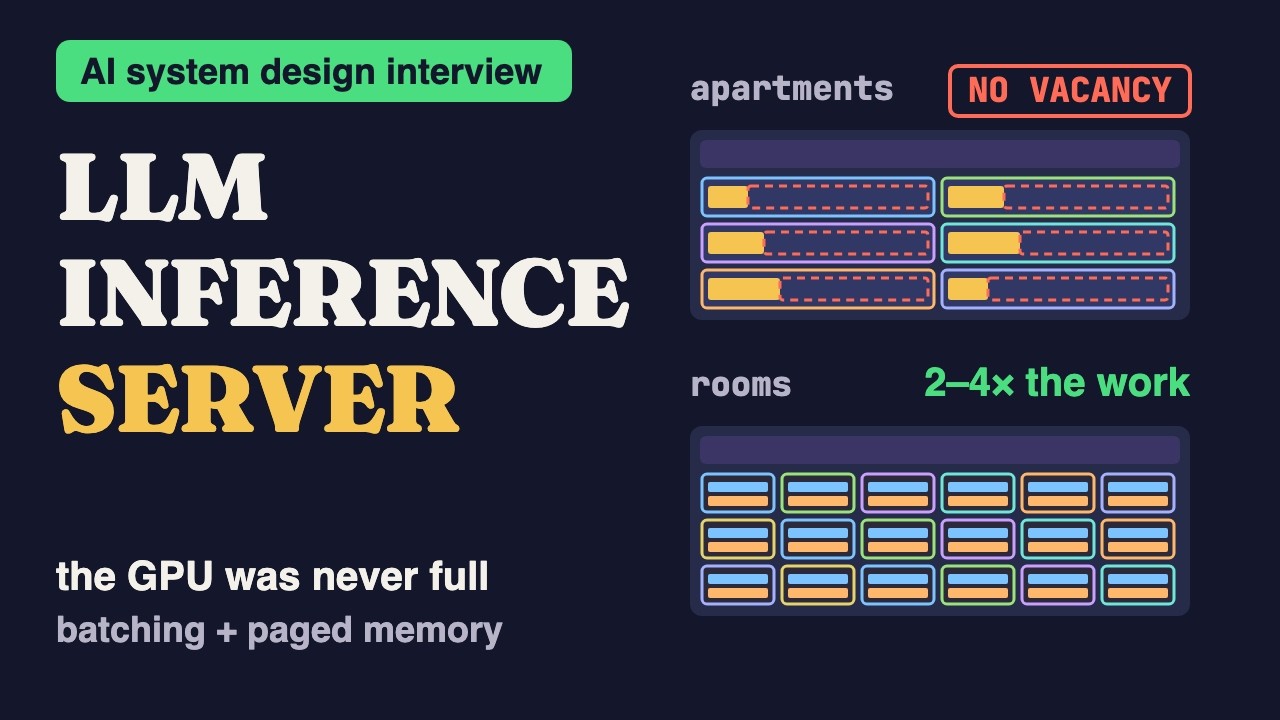
The building was never full — it was reserved

The interactive build above lays out the serving stack: prefill and decode, continuous batching, the paged KV cache, preemption, prefix caching, tensor parallelism and autoscaling. This film follows one question into the GPU at nine at night, finds a chip that “ran out of memory” with most of that memory empty, and then runs the two algorithms that fix it — the scheduler loop and the block allocator — line by line as pseudo code, while the building obeys them.

  • See why it breaks: a static batch waits on its longest answer, and whole-answer reservations leave most of the KV-cache memory empty — only 20–40% held real notes in the systems the PagedAttention paper measured.
  • Take it into the interview: write the continuous-batching loop and the paged allocator from memory, then name what each fix costs — slower tokens per person, special attention code, preemption work, a warm pool paid to wait.

Where an interviewer pokes next

Getting the boxes right is the easy half. These are the questions that separate a candidate who drew the diagram from one who has run the thing. Answer each one out loud before you open it.

  1. A sequence gets preempted when KV memory runs out. Does it restart from token 0, or resume where it left off?

    It depends on what the scheduler chose to do with the evicted KV state: if the state was swapped out to CPU memory rather than discarded, the sequence resumes from where it was once memory frees up — slower than staying resident, but not from scratch. If the state was simply dropped (cheaper, no swap overhead), the sequence has to recompute its prefill from the start. Production schedulers usually swap for short preemptions and only fully drop under sustained, severe pressure, because recomputing a long prefill is expensive.

  2. Continuous batching mixes a 50-token request with a 4000-token one. Does the long one hog memory and starve the short ones?

    Yes, proportionally — KV cache memory scales with sequence length, so one very long generation can consume the memory budget of many short ones combined, capping how many total sequences fit in a batch regardless of how "few" requests are technically running. This is exactly why paged attention’s fixed-block allocation matters: it lets the scheduler admit and evict at block granularity instead of needing one long sequence’s worst case reserved up front.

  3. How would speculative decoding — a small draft model guessing several tokens for the big model to verify at once — interact with continuous batching?

    It adds a second, smaller model into the batch scheduler’s accounting: the draft model runs ahead generating candidate tokens, and the main model verifies a chunk of them in one parallel step instead of one token at a time — when the draft guesses right, decode effectively speeds up for that sequence. The scheduler now has to budget GPU time and KV memory for both models simultaneously, and batching logic has to handle variable "tokens produced per step" per sequence instead of a clean one-token-per-step assumption.

  4. Tensor parallelism needs fast interconnect between GPUs. What actually breaks if you shard a model across GPUs on slow interconnect (say, across separate machines without NVLink)?

    Every layer of the forward pass requires the sharded GPUs to synchronize and exchange partial results, so slow interconnect turns tensor parallelism’s per-layer communication into the bottleneck — you can end up GPU-idle waiting on network transfers more than you’re compute-bound, which can make a "sharded" model SLOWER than a smaller one that fits on a single device. This is why tensor parallelism is typically kept within a single high-bandwidth node (NVLink), and pipeline parallelism (which communicates far less often, only between stages) is preferred for splitting across separate machines.

  5. How does scheduling change when one GPU pool serves several different models instead of one?

    Continuous batching assumes all in-flight sequences share one model’s weights and can be batched into the same forward pass — different models can’t share a batch step, so a multi-model fleet either partitions GPUs per model (simpler, but loses the flexibility to shift capacity between models on demand) or uses a scheduler that can rapidly swap which model’s weights are resident, trading some latency for better overall GPU utilization across an uneven mix of model demand.

Check yourself — the answers, and why

Eight steps in, these are the calls you should be able to make cold. Pick one, then read why.

  1. Continuous (in-flight) batching beats static batching because…

    Static batches stall on the longest sequence; continuous batching slots new requests in and drops finished ones each step, keeping GPUs saturated.

  2. The KV cache makes decode…

    Caching per-token key/value state means a new token reuses prior work, turning O(n²) recomputation into O(n).

  3. Time-to-first-token is dominated by…

    Prefill processes the whole prompt before the first output token; decode then governs tokens/sec.

  4. You should autoscale an inference fleet on…

    GPU saturation and queue depth predict rising latency; CPU metrics miss it, and raw request count ignores token length.

  5. The KV cache runs out of room with too many long sequences active. What does the scheduler do?

    Memory pressure becomes a scheduling decision: preemption (with swap-and-resume where possible) keeps the fleet serving instead of failing outright or corrupting in-flight sequences.

How you’d open this design in an interview

Before any boxes: agree what it must do, pin the qualities that shape everything, then build — naming each trade-off as you make it. The walkthrough above is that exact order.

What it must do

Agree on these before drawing a single box.

  • Serve + stream: take a prompt, admit it, and stream tokens back — optimizing time-to-first-token.
  • Absorb spikes: a request queue buffers bursts and sheds load rather than stampeding the GPUs.
  • Keep GPUs full: continuous batching adds and retires sequences every decode step.
  • Cheap tokens: a paged KV cache reuses attention state so decode is linear, not quadratic.
  • Fit + scale: tensor-shard big models across GPUs; autoscale replicas on GPU pressure.

The qualities that shape everything

Each one names the mechanism that buys it.

Fast time-to-first-token
A router admits and routes to a GPU replica with capacity and streams tokens back — the path is built around streaming, and TTFT is the metric that matters.
Spiky demand on a fixed GPU fleet
A request queue decouples arrival rate from service rate, absorbing bursts and shedding load ("busy, retry") instead of stampeding or starving the workers.
Keep expensive GPUs saturated
Continuous (in-flight) batching runs all active sequences each decode step, retiring finished ones and slotting new arrivals in immediately.
Make each token cheap and concurrency dense
A KV cache reuses per-token attention state (decode goes O(n), not O(n²)), and paged attention stores it in fixed blocks so many sequences pack into GPU memory.
Run a model bigger than one GPU
Tensor-shard each layer’s weights across several GPUs over fast interconnect so they compute a forward pass as one logical worker.
Hold latency as demand swings
An autoscaler watches queue depth and GPU utilization, adding/removing replicas and keeping a warm pool because GPU starts are slow.

The trade-offs you say out loud

Senior signal isn’t the boxes — it’s naming what you gave up and why it was the right price.

Fresh inference behind a router over a CDN cache of common answers

Generations are dynamic and rarely identical, so caching whole answers barely helps; the expensive part is fresh inference, which a router admits and routes to a GPU with capacity.

A request queue over spinning up a GPU per request

GPUs take minutes to provision and cost too much to hold per request; a queue absorbs bursts so a fixed fleet stays fed, with admission control to shed load gracefully.

Continuous batching over static batches

A static batch stalls on its longest sequence while new arrivals wait for it to drain; adding and retiring sequences every step keeps the GPU full regardless of the length mix.

A paged KV cache over recomputing attention every token

Recomputing all prior tokens per new token is quadratic waste; caching per-token key/value state makes decode linear, and paging it in fixed blocks packs many sequences into GPU memory.

Autoscale on GPU pressure over provisioning for peak

Sizing for peak idles expensive GPUs most of the day; scaling on queue depth and GPU utilization with a warm pool matches capacity to demand without cold-start stalls.

The answer, out loud

What a strong answer to “Design an LLM Inference Server” sounds like, first question to last trade-off. It is about 7 minutes of talking; the whiteboard and the interviewer fill the rest of the 45. Read it aloud once, then close the page and give it yourself.

  1. 0–3 min

    Pin down what “serving” means

    Before I draw anything, I want to agree on what we’re serving. Users send a prompt and read the answer as it streams back, so I’ll treat time-to-first-token as the number users feel and tokens per second as the number the business pays for. The fleet is a fixed set of GPUs that cost dollars an hour and take minutes to add. So the real question is: how do we keep scarce, expensive GPUs full while every user still gets a fast first token? Everything I build next is an answer to that.

  2. 3–8 min

    The skeleton, and the shock absorber

    The skeleton is a client, a router and the GPU workers. The router authenticates, applies rate limits, picks a replica with room, and then holds that connection open and streams tokens out as they are produced. Someone usually asks about putting a cache in front, and I’d argue against it here: two people almost never send me the same prompt word for word, and the money goes on producing the answer, not on shipping it. What I do want in front of the workers is a queue. Demand arrives in bursts and the GPU count doesn’t move on that timescale, so without a buffer a spike stampedes the fleet and the quiet hour after it wastes the same fleet. A queue lets the burst wait instead. It also gives me one place to say no — when it’s deeper than the fleet can work through before those people have given up anyway, I’d rather turn them away in a few milliseconds and tell them when to come back than take work I already know I’ll throw away.

    Built in step 2: Put a queue in front of the GPUs
  3. 8–14 min

    How a token is actually made

    Now I need to say how the model computes, because it drives every decision after this. Generation is two phases. Prefill runs the whole prompt through the model in one parallel pass — it’s compute-bound, and it sets time-to-first-token. Decode then produces one token per step, each depending on the last — it’s memory-bandwidth-bound, and it sets tokens per second. The two scale differently, so I’ll tune them separately rather than talk about “latency” as one number.

    Built in step 3: Prefill, then decode
  4. 14–22 min

    Keep the GPUs full

    One decode step for one sequence uses a sliver of the GPU, so batching is where the money is. Static batching — wait for N requests, run them to the end together — stalls the whole batch on its longest answer while new arrivals wait. I’d use continuous batching: at every decode step the scheduler runs all active sequences, retires the ones that just finished and slots waiting ones in immediately, so the GPU stays saturated whatever the length mix. The cost is that a bigger batch nudges any single request’s latency up, and I’d name that as the central trade-off of the whole design.

    Built in step 4: Continuous batching
  5. 22–30 min

    Memory is the real limit

    Attention looks back over every earlier token, so without a cache each new token recomputes the whole sequence — quadratic. A KV cache keeps each token’s key and value state in GPU memory, which makes decode linear. But that cache is now what limits concurrency: how many sequences I can batch is mostly a KV-memory question. Reserving each answer’s worst-case length up front leaves most of that memory empty — the PagedAttention paper measured only 20 to 40 percent of it holding real state. So I page it: fixed-size blocks, allocated as a sequence grows, like virtual memory. When memory still runs out, the scheduler preempts lower-priority sequences — swapping their state out to resume later, or dropping it and recomputing the prefill — so memory pressure becomes a scheduling decision, not an outage.

    Built in step 5: The KV cache and paged attention
  6. 30–36 min

    Fit the model, then ride the demand

    If the weights don’t fit on one GPU, I tensor-shard each layer across several GPUs inside one node, over fast interconnect, so they act as one worker. Across machines I’d rather use pipeline parallelism, because tensor parallelism synchronizes on every layer and a slow link turns that into the bottleneck. For demand: provisioning for peak idles GPUs most of the day, and provisioning for average melts at peak — a queue is buffering, not capacity. So an autoscaler watches queue depth and GPU and KV-cache utilization, not CPU, and keeps a warm pool because GPU starts are slow. Under extreme load it sheds, or routes overflow to a smaller, faster model.

    Built in step 6: Shard the weights across GPUs
  7. 36–42 min

    What I’d watch, and how it fails

    On the dashboard: time-to-first-token, tokens per second, GPU utilization and KV-cache headroom, because those four drive both batching and scaling. The two failures I’d plan for first. The queue floods and time-to-first-token climbs for everyone — the answer is shedding, warm replicas and overflow to a smaller model. Or the mirror image of that: the fleet stops admitting anyone while the request count on the dashboard looks comfortable, because what ran out was memory per live sequence, not slots. That one I’d fix by letting the scheduler set a long sequence aside a piece at a time and bring it back later, which is only something paging leaves me able to do.

  8. 42–45 min

    Close on the trade-off

    To close, I’d restate the design in one breath: a router and a queue in front, prefill and decode treated as different problems, continuous batching over a paged KV cache, sharded weights, and autoscaling on GPU pressure. Every one of those knobs trades latency against throughput. With more time I’d go to speculative decoding and to serving several models from one pool next, because both break assumptions I’ve leaned on — one token per step, and one model per batch.

What this teaches

Learn AI system design by building an LLM inference serving system step by step. An interactive guide covering the request queue, the prefill/decode split, continuous batching, the KV cache and paged attention, tensor sharding across GPUs, autoscaling on GPU pressure, and the latency-versus-throughput trade-offs of serving a model at scale.

Key takeaways

  • Router + stream — admit, route, stream tokens — optimize TTFT
  • Request Queue — shock absorber between spiky demand and fixed GPUs
  • Prefill / decode — parallel prompt pass, then one token per step
  • Continuous batching — add/retire sequences each step — GPUs stay full
  • KV cache + paging — cheap tokens, dense concurrency, memory-bound
  • Tensor sharding — split big models across GPUs to fit and scale
  • Autoscaler — scale on queue depth + GPU util, keep warm pools
  • Latency vs throughput — the trade-off every knob above is balancing

Concepts covered

  • Why is serving an LLM hard?
  • A client, a router, a model
  • Put a queue in front of the GPUs
  • Prefill, then decode
  • Continuous batching
  • The KV cache and paged attention
  • Shard the weights across GPUs
  • Autoscale on GPU pressure
RUN IT YOURSELF

Why batching wins: forward passes

An LLM server batches many requests into one expensive GPU forward pass — that is where throughput comes from. This sketch counts the forward passes for different batch sizes, in real Python, running live. Edit the numbers and hit Run.

HOW TO READ THE CODE — 4 IDEAS
  1. Each forward pass through the model is expensive; you want as few as possible.
  2. Batching serves many requests in a single pass (step 2).
  3. Greedily fill each batch up to max_batch (step 1); the last one takes the remainder.
  4. Fewer passes = higher throughput — though bigger batches add a little latency.
CPython · WebAssembly
RUN IT YOURSELF

Out of KV memory with half the pool allocated and empty

One burst of 24 requests, one 2,048-slot KV pool, and the same continuous-batching loop run twice — once reserving each sequence prompt + MAX_TOKENS contiguously, once handing it 16-token pages from a shared pool. It prints how many sequences fit, what share of the allocated memory is holding real tokens, how the pool splits three ways at the moment the server refuses a waiting request, and the cap below which reservation is the better allocator. Change MAX_TOKENS, hit Run, and watch both rows move.

HOW TO READ THE CODE — 5 IDEAS
  1. Same pool, same workload, same scheduler: reservation held 3 sequences at once, paging held 14. How many requests you can batch is a KV-memory question (step 5), and the answer is set by the shape of the allocation, not the size of the device.
  2. Of the reserved memory, only 39.2% was ever holding a real token, against 97.1% paged — the same 20–40% band the PagedAttention paper measured. At the median refusal the pool was 36% live, 52% allocated and empty, 12% free: out of memory and half idle in the same instant. Those are shares of the device, so they survive changing its size; the stall counters on the next line do not.
  3. A reservation is sized by the max_tokens the client declared, which is a ceiling, not a forecast (step 2) — so raising the cap to 1024 without changing a single answer drops reservation from 3 sequences to 1 and its occupancy to 21.4%. The paged row does not move, and the reason is on the line above it: paging sizes allocation from tokens that exist, so the cap reaches it only by truncating an answer, and at 512 nothing is truncated. Type MAX_TOKENS = 128 and the paged row moves too.
  4. Paging is not free and the file prints the invoice: every sequence carries up to 15 slots of part-filled page, and when the pool ran dry the scheduler preempted 3 times, throwing away a prefill to recompute later — memory pressure as a scheduling decision (step 5). Reservation never preempts; buying the worst case up front is exactly what guarantees it progress.
  5. Paging is not unconditionally better, and the last line is the file searching for where it stops being better: below a cap of 32 tokens — two pages — reservation admits more, because the 20% watermark paging holds back costs more than a cap that short costs reservation. That number is scanned for, not asserted, so it moves when you move BLOCK or the watermark.
CPython · WebAssembly
built to be reasoned about, not memorized — make the calls, flood the queue, run the quiz.
Finished this one? 0 / 61 AI System Designs done

Explore the topic

See this alongside everything else on the same subject — handbooks, system designs, challenges and tools, in one place.

More AI System Designs